Visualization

exaqt.visualization draws a state vector, and can keep a window open that follows a state while you evolve it:

• plotstate returns a matplotlib figure of a state at one moment.
• StateWindow is a window that moves gradually to the new state each time you call update().

Both read the state in place and never copy it (see Memory and speed).

Installation

The plots need matplotlib, which the base install leaves out. The visualization extra adds it:

pip install 'mimiq-exaqt[visualization]'

The extra installs mimiqcircuits[visualization], so the plots use the same matplotlib version range and the same MIMIQ style as mimiqcircuits.visualization.plothistogram. import exaqt alone never loads matplotlib; the module is imported only when you ask for it:

from exaqt.visualization import plotstate, StateWindow

A StateWindow also needs a GUI toolkit for matplotlib to draw into; see Windows and backends. plotstate does not.

Plotting a state: plotstate

import mimiqcircuits as mc
from exaqt import ExaqtState, evolve
from exaqt.visualization import plotstate

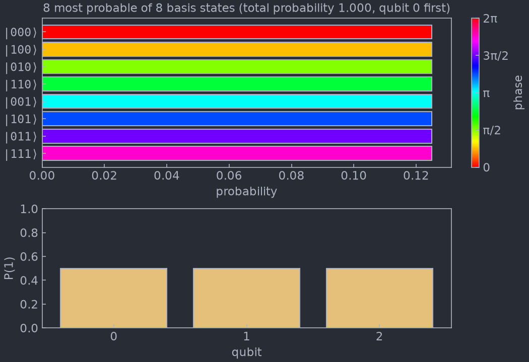
# H on every qubit gives all 8 basis states the same probability, 1/8.
# T, S and Z then add a phase of π/4, π/2 and π for each qubit set to 1,
# so basis state i (qubit 0 as the lowest bit) ends up with phase i·π/4.
c = mc.Circuit()
for q in range(3):
    c.push(mc.GateH(), q)
c.push(mc.GateT(), 0)
c.push(mc.GateS(), 1)
c.push(mc.GateZ(), 2)

state, _ = evolve(ExaqtState.zero(3), c)
fig = plotstate(state)
fig.savefig("phases.png")

Reading the plot

Top panel: the most probable basis states. One bar per basis state, most probable first.

• The bar length is the probability |⟨i|ψ⟩|².
• The bar colour is the phase of the amplitude, read on the colour bar on the right. Phase is cyclic, so the colour map is too: a phase just below 2π and a phase just above 0 get nearly the same colour. Two states with the same probability and different phases, as above, are told apart only by colour.
• States of equal probability come in basis order.
• The title gives how many states are listed and the total probability they carry. When that total is well below 1, the state is spread over more basis states than the plot lists.

Bottom panel: P(1) for each qubit. The probability of measuring 1 on each qubit on its own. It stays readable when 2**n is far too many amplitudes to list: a qubit at 0 or 1 is in a definite state, a qubit near 0.5 is maximally uncertain.

Bitstrings list qubit 0 first, as mimiqcircuits.BitString does: |100⟩ is qubit 0 set, the others clear. That is the basis state of index 1, since qubit 0 is the lowest bit of the index.

Options

Argument	Default	Effect
num_states	15	Maximum number of basis states listed.
mimiqstyle	True	Draw in the MIMIQ matplotlib style; False keeps your active style.

In notebooks and scripts

plotstate returns a matplotlib.figure.Figure.

• In a notebook, a call on the last line of a cell displays the figure once. Assigned to a variable (fig = plotstate(state)), it displays nothing until you show fig.
• In a script, save it with fig.savefig(...), or open it with matplotlib.pyplot.show().

Watching a state evolve: StateWindow

StateWindow opens a window on a state and redraws it only when you call update(). Each update reads the state as it is then, and moves the picture there gradually over about a second. Between two updates you evolve the state by as many gates as you like, so you choose when to look.

import matplotlib.pyplot as plt
import mimiqcircuits as mc
from exaqt import ExaqtState, evolve
from exaqt.visualization import StateWindow

state = ExaqtState.zero(4)
window = StateWindow(state)          # opens on |0000>

# One layer: an RY on every qubit, then a CX ladder.
layer = mc.Circuit()
for q in range(4):
    layer.push(mc.GateRY(0.4), q)
for q in range(3):
    layer.push(mc.GateCX(), q, q + 1)

for _ in range(5):
    evolve(state, layer)             # evolve in place, any number of gates...
    window.update()                  # ...then animate to where the state is now

plt.show()                           # keep the window open at the end

The window keeps a reference to state and reads it at every update(), so evolve that same object in place, as evolve does. It never modifies the state.

What an update animates

The window shows what plotstate shows. During an update:

• bars grow or shrink to their new probability and slide to their new rank;
• bar colours turn to the new phase, the short way round the colour wheel;
• basis states that leave the list fade out where they stand, and those that join it fade in at their new rank;
• the P(1) bars and the probability axis move to their new values.

The animation follows the clock: if the window redraws slowly it shows fewer frames, but still takes the time asked for.

update()

window.update()                      # animate over the window's duration
window.update(duration=0.3)          # a quicker transition
window.update(duration=0)            # jump straight to the new picture

update() always reads the state the window was created on. To watch another state, open another window.

Argument	Default	Effect
duration	the window's	Length of the animation in seconds; 0 jumps straight to the new picture.

StateWindow(state, num_states=15, mimiqstyle=True, duration=1.0) takes the same num_states and mimiqstyle as plotstate, and duration sets the default length of an update.

update() raises RuntimeError once the window has been closed; open a new StateWindow to continue.

Windows and backends

A window needs an interactive matplotlib backend, which in turn needs a GUI toolkit installed. The toolkit belongs to your environment, so the visualization extra does not install one:

• Tk comes with most Python installs (python.org, Windows, conda, most Linux distributions), and matplotlib uses it with no setup.
• Qt works with pip install PyQt6 or pip install PySide6. Use it where Python was built without Tk, as Homebrew's is.

Where the window is drawn from matters:

• In a script, the window repaints only while update() runs. Between two updates it shows the last frame but does not respond to resizing. End the script with plt.show() to keep the window open and responsive, or pause with plt.pause(seconds) between updates.
• In Jupyter, run %matplotlib qt (or %matplotlib tk) before creating the window. The notebook's default inline backend draws static images, which cannot animate.
• With a non-interactive backend (Agg, inline), nothing opens and update() redraws the figure in one step. Nothing fails, so the same code runs in tests and on headless machines.

Memory and speed

Neither plotstate nor StateWindow.update() copies the state vector. Both read it through ExaqtSV.summary(k), one parallel pass that collects the k most probable basis states and P(1) of every qubit together.

The extra memory is proportional to num_states, not to 2**n, and a plot costs about as much as reading the state once: 0.25 s on a 28-qubit state (4 GiB). A StateWindow makes that pass at every update(), and none in between.

The same call gives you the numbers without plotting anything:

# The 5 most probable basis states (most probable first), P(1) of every
# qubit, and the squared norm, all from one pass over the state.
indices, amplitudes, p1, norm2 = state.q.summary(5)

Limits

• Dynamic qubits. A state built with dynamic_qubits=True is refused with ValueError: its buffer is stored in a permuted qubit order, so bitstring labels would name the wrong qubits.
• GPU state vectors. Only CPU states can be plotted for now: a state on an ExaqtSVGpu is refused with TypeError.