Visualization

tensorweaver.visualization draws the entanglement structure of an MPS: how large each bond has grown, how much entanglement each cut carries, and what the bond dimension cap cut off. It can also keep a window open that follows a state while you evolve it:

• plotbonds plots the bond dimension and the entanglement entropy of every cut.
• plotschmidt plots the Schmidt spectrum of one cut.
• BondWindow is a window that moves gradually to the new bond structure each time you call update().

They answer the question that decides whether an MPS run can be trusted: is the bond dimension large enough for this circuit, and if not, where does it fall short? See Cutoffs and bond dimension for the knobs involved.

Installation

The plots need matplotlib, which the base install leaves out. The visualization extra adds it:

pip install 'mimiq-tensorweaver[visualization]'

The extra installs mimiqcircuits[visualization], so the plots use the same matplotlib version range and the same MIMIQ style as mimiqcircuits.visualization.plothistogram. import tensorweaver alone never loads matplotlib; the module is imported only when you ask for it:

from tensorweaver.visualization import plotbonds, plotschmidt, BondWindow

A BondWindow also needs a GUI toolkit for matplotlib to draw into; see Windows and backends. The two plots do not.

Every function takes a TwState, such as the one TwSimulator.evolvezerostate returns, or a bare MPS.

Bond numbering

The plots number bonds as MPS.bond_dim and MPS.schmidt_values do: bond k is the cut between qubits k-1 and k. An n-qubit chain has interior bonds 1 to n-1; bonds 0 and n are its open ends, always of dimension 1, and are not drawn.

MPS.all_entropies() counts the other way, its element k being the cut between qubits k and k+1. The plots take care of the offset, so the entropy drawn at bond k is always that of the cut between k-1 and k.

Bond dimensions and entropies: plotbonds

import mimiqcircuits as mc
import tensorweaver as tw
from tensorweaver.visualization import plotbonds

# A 12-qubit brickwork: RY rotations, then CX bricks on alternating pairs.
# Six layers entangle the middle of the chain more than χ = 4 can hold.
c = mc.Circuit()
for layer in range(6):
    for q in range(12):
        c.push(mc.GateRY(0.5 + 0.1 * q), q)
    for q in range(layer % 2, 11, 2):
        c.push(mc.GateCX(), q, q + 1)

state, fidelity = tw.TwSimulator(bonddim=4, strict_bonddim=False).evolvezerostate(c)
print(fidelity)                      # 0.9954...: truncation discarded some weight

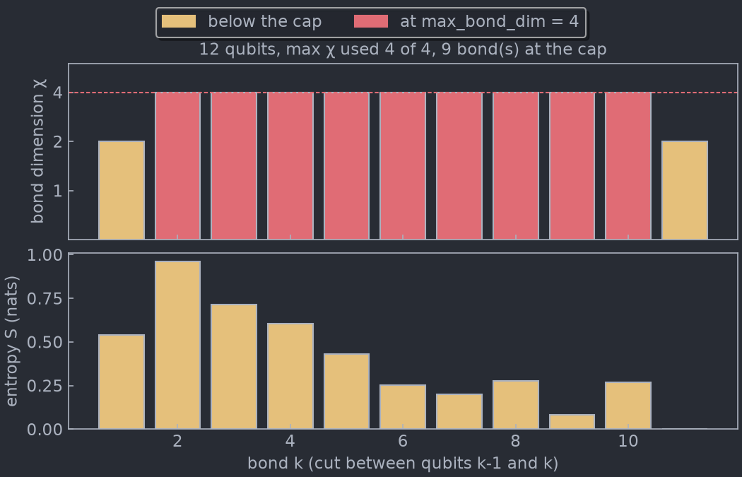
fig = plotbonds(state)
fig.savefig("bonds.png")

Reading the plot

Top panel: bond dimension χ. One bar per bond, on a log-2 axis, since bond dimensions grow by doublings: χ = 2 and χ = 256 both stay readable. The dashed line is max_bond_dim, the cap set by TwSimulator(bonddim=...).

• A red bar has reached the cap. It holds as many Schmidt values as the simulator allows, so any further weight on that cut was discarded. Red marks where truncation can happen, not where it did: a state can fit its cap exactly, as a GHZ state does at χ = 2, and then nothing is lost. The fidelity returned with the state, and plotschmidt, tell how much it cost.
• A bar below the cap was not limited by bonddim, though sv_cutoff can still have dropped small Schmidt values there.
• χ = 1 means the two sides of the cut are not entangled at all.
• Near the ends of the chain χ is bounded by the chain itself: bond k can never exceed 2**min(k, n-k) for qubits.

The title gives the largest χ in use and how many bonds sit at the cap. Several bonds at the cap and a fidelity below 1 mean the run needs a larger bonddim.

Bottom panel: entanglement entropy S. The von Neumann entropy of each cut, in nats: S = -Σ λᵢ² ln λᵢ² over the Schmidt values λᵢ. Zero is a product cut. One Bell pair across a cut gives ln 2 ≈ 0.693, and a cut of χ Schmidt values carries at most ln χ. The entropy says how much entanglement a bond carries, where χ only says how much room it takes.

The spectrum of one cut: plotschmidt

from tensorweaver.visualization import plotschmidt

# Bond 6, the middle of the chain above, is at the cap.
fig = plotschmidt(state, 6)
fig.savefig("bond6.png")

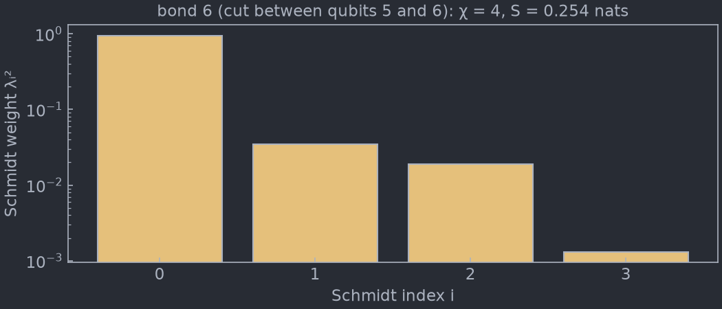
Each bar is a Schmidt weight λᵢ², the probability carried by one Schmidt vector of the cut, largest first, on a log scale. The weights of a normalized state add up to 1. The title repeats χ and the entropy of the cut.

• A spectrum that falls off fast, as here, means the cut is well represented: the smallest weight kept is about 10⁻³, so what the cap cut off beyond it was small.
• A spectrum still high where it ends means the cap is cutting off weight that matters, and a larger bonddim would change the result.

Reading the spectrum moves the MPS orthogonality center to bond. That changes the MPS gauge, not the state: no amplitude changes.

In notebooks and scripts

plotbonds and plotschmidt return a matplotlib.figure.Figure.

• In a notebook, a call on the last line of a cell displays the figure once. Assigned to a variable (fig = plotbonds(state)), it displays nothing until you show fig.
• In a script, save it with fig.savefig(...), or open it with matplotlib.pyplot.show().

Both take mimiqstyle=True by default; mimiqstyle=False draws in your active matplotlib style instead.

Watching the bonds grow: BondWindow

BondWindow opens a window on a state and redraws it only when you call update(). Each update reads the state as it is then, and moves the picture there gradually over about a second. Between two updates you evolve the state by as many gates as you like, so you choose when to look.

import matplotlib.pyplot as plt
import mimiqcircuits as mc
import tensorweaver as tw
from tensorweaver.visualization import BondWindow

sim = tw.TwSimulator(bonddim=16, strict_bonddim=False)
state = sim.build_state(20)          # |0...0>: every bond at χ = 1
window = BondWindow(state)

# One layer: an RY on every qubit, then a CX ladder. Compile it once.
layer = mc.Circuit()
for q in range(20):
    layer.push(mc.GateRY(0.7), q)
for q in range(19):
    layer.push(mc.GateCX(), q, q + 1)
step = sim.compile(layer)

for _ in range(6):
    sim.evolve(state, step)          # evolve in place, any number of gates...
    window.update()                  # ...then animate to where the state is now

plt.show()                           # keep the window open at the end

TwSimulator.build_state(n) gives a fresh |0…0⟩ state, and TwSimulator.evolve(state, compiled) evolves it in place by a circuit that TwSimulator.compile prepared. The window keeps a reference to state and reads it at every update().

What an update animates

The window shows what plotbonds shows. During an update:

• bond dimensions move to their new values along the log-2 axis, so a bond going from 2 to 8 passes through 4 half way;
• bars fade to red as they reach the cap, and back if they leave it;
• entropies and the entropy axis move to their new values;
• the title changes to the new state at the end.

The animation follows the clock: if the window redraws slowly it shows fewer frames, but still takes the time asked for.

update()

window.update()                      # animate over the window's duration
window.update(duration=0.3)          # a quicker transition
window.update(duration=0)            # jump straight to the new picture

update() always reads the state the window was created on. To watch another state, open another window.

Argument	Default	Effect
duration	the window's	Length of the animation in seconds; 0 jumps straight to the new picture.

BondWindow(state, mimiqstyle=True, duration=1.0) takes the same mimiqstyle as plotbonds, and duration sets the default length of an update.

update() raises RuntimeError once the window has been closed; open a new BondWindow to continue.

Windows and backends

A window needs an interactive matplotlib backend, which in turn needs a GUI toolkit installed. The toolkit belongs to your environment, so the visualization extra does not install one:

• Tk comes with most Python installs (python.org, Windows, conda, most Linux distributions), and matplotlib uses it with no setup.
• Qt works with pip install PyQt6 or pip install PySide6. Use it where Python was built without Tk, as Homebrew's is.

Where the window is drawn from matters:

• In a script, the window repaints only while update() runs. Between two updates it shows the last frame but does not respond to resizing. End the script with plt.show() to keep the window open and responsive, or pause with plt.pause(seconds) between updates.
• In Jupyter, run %matplotlib qt (or %matplotlib tk) before creating the window. The notebook's default inline backend draws static images, which cannot animate.
• With a non-interactive backend (Agg, inline), nothing opens and update() redraws the figure in one step. Nothing fails, so the same code runs in tests and on headless machines.

Cost

The plots read little of the state. Bond dimensions are read directly. The entropies move the orthogonality center along the chain once, taking one SVD of a single site tensor per bond, and plotschmidt does the same for one cut. The MPS is never copied as a whole. A BondWindow makes the same reads at every update(), and none in between.

A state from a TwSimulator(usegpu=True) is brought back to host memory before it is read, as for any other read-out of the state.